This article is a basic introduction. Readers will need a good understanding of the fundamentals of calculus; experience with programming is recommended. Anyone with a background in math or physics will probably find all of the points made quite trivial.

In essence, I will be summarizing Nils Berglund's How to simulate the wave equation. If you enjoy this article, I think you will find his simulations quite interesting.

\(***\)

This is Bob:

👷

Bob is a civil engineer who has been tasked with creating a breakwater to protect a remote area against flooding by large waves, which are somewhat frequent there. Bob has done this before; he plans out a simple embankment and then heads to bed. Since there's nothing important in the area, a few of the larger waves crossing the dike shouldn't hurt anyone.

Unfortunately Bob's superiors forgot to mention that there's actually a nuclear power plant only a few meters away from the coast. Nobody knows who was responsible for choosing the site or overseeing construction. Anyway, the embankment Bob has designed isn't going to cut it — and he doesn't have the budget to build a bigger one.

Instead Bob will have to find a way to prevent the larger waves of reaching it in the first place. He decides to place poles in front of the dike to break the waves, reducing their height. However the tribulations of our engineer aren't over yet; with these high stakes he needs to be sure that his solution will actually work, and he should probably find a way of choosing the best shape for the poles instead of guessing.

In this case there aren't any simple calculations to be done — the only way to know is to build and test it. But Bob has to hand in his design by Thursday! He doesn't have the time to construct a test dike or even a small-scale model of the dike. The only possible thing left to do is run a fluid simulation. Bob makes a quick 3D model and uploads it to the server that runs the expensive CFD software.

Bob's bad week isn't over yet; in fact it just got worse. The server site has just been flooded by a large wave. Bob realizes that people should perhaps stop building things next to water. Bob needs a break. Let's give him a hand and try to do his simulations for him.

CFD (Computational Fluid Dynamics) software is complicated and performance-intensive and is an object of ongoing research. Water is a lot more complex than just waves moving through a medium; instead we're going to build something simpler by just focusing on the wave behaviours. These are more abstract and can be found in many places, for example in air or light or badly constructed bridges or even a stadium audience.

An audience wave is actually a very good example by which we can understand what waves fundamentally are. For an audience wave to occur, audience members simply need to stand up or sit down so that they are matching what their neighbours are doing, i.e. they tend towards the average state of their neighbours. We should also note that audience members have inertia; they can't magically snap to any position. These two properties can be found in many, many places, which is why waves are such a frequent phenomenon.

A simpler example might be found in the contraption you can see in the diagram below. We mount rails to a table and place carts on them, so that they can only move back and forth. We then connect each cart to its neighbours via springs so that it is accelerated towards the positions of its neighbours.

Here's how the forces would act on a random setup:

Next we'll try to replicate the behaviour of this system. Every cart has a value \(u\) that represents its vertical position; \(u=0\) is the center. For simplicity, we'll assume that all carts have the same mass, and that there is no air resistance or friction with the rails. Since the carts are connected by springs, we can calculate the forces being applied with Hooke's Law, which states that the larger the distance \(\Delta u\) between a cart and the value of its neighbour, the more it is accelerated toward that value. The acceleration applied to a cart \(u\) by each neighbouring cart \(u_N\) is:

The coefficient \(q>0\) describes the strength of the acceleration and is determined by how stiff the springs are and how heavy the carts are.

Based on this we can write a simple python script simulating a row of carts:

import numpy as np

# Constants
cart_count = 30
q = 0.2

# Time management
dt = 0.1
t = 0
max_t = 10

# Carts
cartPos = np.array([0.0] * cart_count)
cartVel = np.array([0.0] * cart_count)

# Initial conditions
cartPos[14] = 0.8
cartPos[15] = 0.8

while t < max_t:
    for i in range(cart_count):
        if i > 0:
            cartVel[i] += dt * q * (cartPos[i-1] - cartPos[i])
        if i < cart_count - 1:
            cartVel[i] += dt * q * (cartPos[i+1] - cartPos[i])

    for i in range(cart_count):
        cartPos[i] += dt * cartVel[i]

    t += dt

    print(cartPos)

In this setup, we've pulled up the center carts and then let go.

I've added some boilerplate MatPlotLib code so that we can see the result as an animated graph:

I would call that a success! We've recreated the oscillating behaviour of waves, and we can even see two of them propagating outwards from the center.

In the following I've adapted the script so that we can see the propagation behaviour better.

...

q = 2

...

# Remove initial conditions

while t < max_t:
    for i in range(cart_count):
        if i > 0:
            cartVel[i] += dt * q * (cartPos[i-1] - cartPos[i])
        if i < cart_count - 1:
            cartVel[i] += dt * q * (cartPos[i+1] - cartPos[i])

    for i in range(cart_count):
        cartPos[i] += dt * cartVel[i]
        
    cartPos[0] = 0.5 * np.sin(t)

    ...

Here we're moving the left end back and forth. We can see the resulting sine wave propagate smoothly from left to right.

So far so good, our model works. In order to gain more understanding about what is happening here, our next step is to generalize: We want our model to describe waves as a whole, not just our contraption. There are currently two issues to be solved: Firstly, \(q\) has no meaning outside of springs; we should like to gain some more understanding about what our constants actually represent. Secondly, our model is not resolution independent. If we scale the resolution of our cart model, we're also scaling the wave itself, since all we're doing is adding more carts. Furthermore, not all wave mediums are discretized into individual "carts", instead their resolution is infinite.

When I mention the words "infinite resolution", you might interpret that the way it's meant mathematically: in that our function \(u(x,t)\) accepts \(x \in \mathbb{R}\) instead of \(x=n \Delta x \; (n \in \mathbb{Z})\). Or you might take it literally in that \(\Delta x\) goes toward zero, similarly to how it does in the derivative: \[u(x,t) = \lim\limits_{\Delta x \to 0} u(n \Delta x,t)\]

To put it another way: The relationship between the physical cart model and the wave function is quite similar to the relationship between the difference quotient and the derivative. Our goal is to convert the spring model into a form that contains derivatives instead of discrete differences.

Let's write out our spring formula in one dimension: \[a_x=q (\Delta u_{x-\Delta x} + \Delta u_{x+\Delta x})\]

For clarity, we'll replace \(u_x\) with \(u(x,t)\) and \(a_x\) with the second temporal derivative: \[\frac{du(x,t)}{dt^2}=q ((\,u(x-\Delta x,t) - u(x,t)\,) + (\,u(x+\Delta x,t) - u(x,t)\,))\]

A quick Mathematical Fun Fact from Bob: The derivative of a function with multiple inputs is called a partial derivative (assuming only one variable changes) and has its own notations, both using a special cursive d: \[ \begin{align*} \text{First derivative:}\quad\frac{du(x,t)}{dt} &\rightarrow \frac{\partial u(x,t)}{\partial t}=\partial_tu(x,t) \\[10pt] \text{Second derivative:}\quad\frac{du(x,t)}{dt^2} &\rightarrow \frac{\partial u(x,t)}{\partial t^2}=\partial_{tt}u(x,t) \end{align*} \] I will be using both notations (those to the right of the arrows) interchangeably from here on.

\[\partial_{tt}u(x,t)=q ((\,u(x-\Delta x,t) - u(x,t)\,) + (\,u(x+\Delta x,t) - u(x,t)\,))\]

This is our fully expanded form. See that \(u(x+\Delta x,t) - u(x,t)\)? If we divide by \(\Delta x\) we'll have a difference quotient, which is precisely what we're aiming for! We can also replace \(u(x-\Delta x,t) - u(x,t)\) with \(-(u(x,t) - u(x-\Delta x,t))\), which switches the minuend and subtrahend, allowing us to form a difference quotient for the right term as well.

\[\partial_{tt}u(x,t)=q \Delta x \left( \frac{u(x+\Delta x,t) - u(x,t)}{\Delta x} - \frac{u(x,t) - u(x-\Delta x,t)}{\Delta x} \right) \]

Purely going off of intuition, the next step would be to convert to a derivative:

\[\frac{f(x+\Delta x)-f(x)}{\Delta x}\simeq f'(x)\]

...if it weren't for the fact that that's not a very good approximation. Let's take a look at an example:

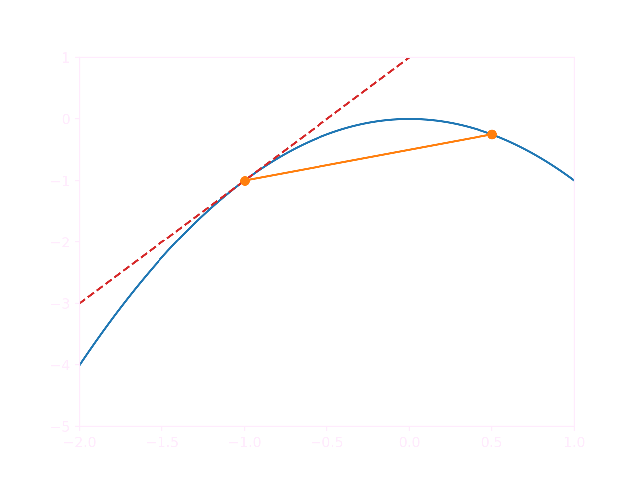
The slope of the difference quotient (in orange) and that of the tangent (in red) are quite far apart. As it turns out, even in simple situations like a quadratic or trigonometric function, the difference quotient isn't necessarily an accurate estimation. A much better solution is to approximate the derivative at the midpoint instead:

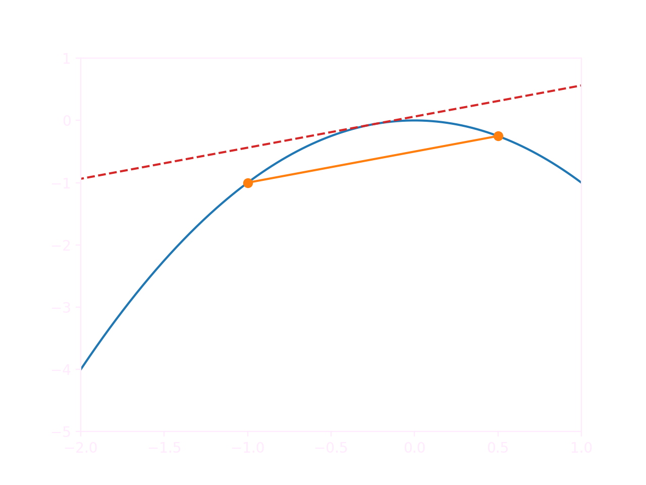
\[\frac{f(x+\Delta x/2)-f(x-\Delta x/2)}{\Delta x}\simeq f'(x)\]

We can prove that this is valid by replacing \(f(x+\Delta x/2)\) and \(f(x-\Delta x/2)\) with the appropriate second-degree Taylor polynomials at \(a=x\).

\[ \begin{align*} \frac{f(x+\Delta x/2)-f(x-\Delta x/2)}{\Delta x} \simeq & \frac{(f(x)+f'(x)(x+\Delta x/2-x)+\frac{f''(x)}{2}(x+\Delta x/2-x)^2)}{\Delta x} \\ &- \frac{(f(x)+f'(x)(x-\Delta x/2-x)+\frac{f''(x)}{2}(x-\Delta x/2-x)^2)}{\Delta x} \end{align*} \]

Another Mathematical Fun Fact from Bob: A Taylor polynomial of a function \(f(x)\) at \(a\) is a method for approximating \(f(x)\) in the area around \(x=a\). The second-degree Taylor polynomial is: \[ f(x) \simeq f(a)+f'(a)(x-a)+\frac{f''(a)}{2}(x-a)^2 \] A second-degree Taylor polynomial is accurate to an almost comical degree if \(x\) and \(a\) are close to each other, which is definitely the case here.

We can now eliminate all terms except \(f'(x)\):

\[ \begin{align*} & \frac{(f(x)+f'(x)(x+\Delta x/2-x)+\frac{f''(x)}{2}(x+\Delta x/2-x)^2)}{\Delta x} \\ & -\frac{(f(x)+f'(x)(x-\Delta x/2-x)+\frac{f''(x)}{2}(x-\Delta x/2-x)^2)}{\Delta x} \\ = & \frac{(f(x)+f'(x)(\Delta x/2)+\frac{f''(x)}{2}(\Delta x/2)^2) - (f(x)+f'(x)(-\Delta x/2)+\frac{f''(x)}{2}(-\Delta x/2)^2)}{\Delta x} \\ = & \frac{(f'(x)(\Delta x/2)) - (f'(x)(-\Delta x/2))}{\Delta x} \\ = & f'(x)\frac{(\Delta x/2) - (-\Delta x/2)}{\Delta x} = f'(x)\frac{2\Delta x/2}{\Delta x} = f'(x) \end{align*} \]

\[\Downarrow\]

\[\frac{f(x+\Delta x/2)-f(x-\Delta x/2)}{\Delta x}\simeq f'(x)\]

... successfully proving that the midpoint derivative is a very good approximation.

We can now apply it to our equation:

\[\partial_{tt}u(x,t)=q \Delta x \left( \frac{u(x+\Delta x,t) - u(x,t)}{\Delta x} - \frac{u(x,t) - u(x-\Delta x,t)}{\Delta x} \right) \]

\[\downarrow\]

\[\partial_{tt}u(x,t) \simeq q \Delta x (\partial_xu(x+\Delta x/2,t) - \partial_xu(x-\Delta x/2,t))\]

We can repeat the process again:

\[\partial_{tt}u(x,t) \simeq q \Delta x ^2 \frac{\partial_xu(x+\Delta x/2,t) - \partial_xu(x-\Delta x/2,t)}{\Delta x}\]

\[\downarrow\]

\[\partial_{tt}u(x,t) \simeq q \Delta x ^2 \partial_{xx}u(x,t)\]

We have reached a solution. It's quite fascinating that we can capture such complex behaviour in a single line.

Bob interjects to point out that this still isn't really resolution independent, since \(\Delta x ^2\) is a coefficient. Instead, we will (for now) replace \(q \Delta x^2\) with the placeholder \(p\). If we allow \(q\) to vary, we can set \(p\) to a constant value.

We can use this equation to either figure out the acceleration of a given wave state, or we can check the validity of a wave function. Let's do that with a simple example. Bob thinks back to his high school days and suggests a cosine wave of the form:

\[u(x,t)=\cos(kx-\omega t)\]

Bob can even remember that \(k\) stands for \(2\pi /\lambda\), representing the inverse of the wavelength, and that \(\omega\) stands for \(2 \pi f\), representing frequency.

We insert our function into the wave equation and apply the chain rule:

\[ \begin{align*} \partial_{tt}\cos(kx-\omega t) &= p * \partial_{xx}\cos(kx-\omega t) \\ \partial_{t}(-\sin(kx-\omega t)(-\omega)) &= p * \partial_{x}(-\sin(kx-\omega t)k) \\ -\cos(kx-\omega t)(-\omega)^2 &= p * ( -\cos(kx-\omega t)k^2) \\ (-\omega)^2 &= p * k^2 \\ p &= \left( \frac{\omega}{k} \right) ^2 \end{align*} \]

Assuming we choose \(p\) correctly, a cosine wave is a valid wave function. (As is any other twice differentiable function \(f(ax-bt)\) !) Additionally, since \(\lambda f=c\) (where \(c\) is the speed of the wave) we can conclude that

\[ p = ( \lambda f ) ^2 = c^2 \]

\(p\) is actually the squared wave velocity. In fact, \(p=c^2\) holds true regardless of what function we're using. The correct and final form of the wave equation is thus

Waves travelling in different directions don't change each other's behaviour, but simply stack on top each other. This means that to derive versions of the wave equation in different dimensions, we simply need to take the sum of the wave equation along each axis: \[ \begin{align*} \text{1D:} & \quad \partial_{tt}u(x,t) &&= c^2 \partial_{xx}u(x,t) \\ \text{2D:} & \quad \partial_{tt}u(x,y,t) &&= c^2 ( \partial_{xx}u(x,y,t) + \partial_{yy}u(x,y,t) ) \\ \text{3D:} & \quad \partial_{tt}u(x,y,z,t) &&= c^2 ( \partial_{xx}u(x,y,z,t) + \partial_{yy}u(x,y,z,t) + \partial_{zz}u(x,y,z,t) ) \end{align*} \]Deriving higher-dimensional wave equations by hand from the cart model produces the same result.

\(***\)

That's the theoretical bit done. Of course Bob doesn't just need the pure maths, he also needs a functioning piece of software. For a practical implementation we will need to do some more work. In order to perform actual simulations, we will want to impose more constraints on \(u(x,t)\); for example we might want to set specific start conditions or place obstacles inside our domain. Describing this as a function lies somewhere in between 'highly challenging' and 'impossible'. Instead, we want to simulate the wave equation step-by-step, always predicting the next state of the system from the current one.

In order to do this we will have to bring our equation back into a discretized form, i.e. one where there is limited resolution. Basically we're working backwards from the wave equation towards our spring model, except that we now know what \(q\) means.

If you recall our approximation method it should quite easy to untangle the partial derivatives: \[ \begin{align*} \partial_{xx}u(x,t) &\simeq \frac{u(x + \Delta x,t) + u(x - \Delta x,t) - 2u(x,t)}{\Delta x ^2} \\[10px] \partial_{tt}u(x,t) &\simeq \frac{u(x,t + \Delta t) + u(x,t - \Delta t) - 2u(x,t)}{\Delta t ^2} \end{align*} \]

\[\downarrow\]

\[ \frac{u(x,t + \Delta t) + u(x,t - \Delta t) - 2u(x,t)}{\Delta t ^2} = c ^2 \frac{u(x + \Delta x,t) + u(x - \Delta x,t) - 2u(x,t)}{\Delta x ^2} \]

In order to find the value of the next state, we solve for \(u(x, t+\Delta t)\):

\[ u(x,t + \Delta t) = 2u(x,t) - u(x,t - \Delta t) + c ^2 \frac{\Delta t ^2}{\Delta x ^2} ( u(x + \Delta x,t) + u(x - \Delta x,t) - 2u(x,t) ) \]

If we keep a copy of the state at \(t - \Delta t\) and at \(t\), we can compute the state at \(t + \Delta t\) and then increment \(t\) by \(\Delta t\), repeating the process as desired. We are effectively calculating the rate of change (the velocity) of the wave from the difference between the two timesteps. Since the velocity is thus implicitly changed when the wave state is changed, this method is equivalent to leapfrog integration.

import numpy as np

# Constants
cell_res = 30
c = 0.5

dx = 1

# Time management
dt = 0.1
t = 0
max_t = 20

# Wave States
previousWave = np.array([0.0] * cell_res)
currentWave = np.array([0.0] * cell_res)
futureWave = np.array([0.0] * cell_res)

# Initial conditions
previousWave[14] = 0.8
previousWave[15] = 0.8
currentWave[14] = 0.8
currentWave[15] = 0.8

fig_num = 0

while t < max_t:
    for i in range(cell_res):
        adjacentSum = 0
        if i > 0:
            adjacentSum += currentWave[i - 1]
        if i < cell_res - 1:
            adjacentSum += currentWave[i + 1]

        futureWave[i] = 2 * currentWave[i] - previousWave[i] \
          + c**2 * dt**2 / (dx**2) \
          * (adjacentSum - 2 * currentWave[i])

    t += dt

    previousWave = currentWave
    currentWave = futureWave
    futureWave = np.array([0.0] * cell_res)

    print(currentWave)

Note that at the boundaries, we are basically setting the value of any cells outside the domain to zero. Here's the result:

In order to guarantee stability, we have to ensure that a wave cannot travel more than one space step in one time step. After all, each cell can only communicate with its neighbours, which means that information can only travel at the speed of one cell per time step. If our wave velocity is higher, chaos ensues; we can only permit wave velocities that are small enough.

\[\begin{align*} c \Delta t &\leq \Delta x \\[5px] c \frac{\Delta t}{\Delta x} &\leq 1 \end{align*}\]

\(c \frac{\Delta t}{\Delta x}\) is commonly abbreviated as \(C\), which is known as the Courant number; the condition that we have found (\(C \leq 1\)) is known as the Courant-Friedrichs-Lewy condition. By extension the discretized wave equation is often written as

\[ u(x,t + \Delta t) = 2u(x,t) - u(x,t - \Delta t) + C ( u(x + \Delta x,t) + u(x - \Delta x,t) - 2u(x,t) ) \]

Finally, we can expand our discretized equation to two or more dimensions.

\[\begin{align*} u(x,t + \Delta t) = 2u(x,y,t) - u(x,y,t - \Delta t) + C ( & u(x + \Delta x,y,t) + u(x - \Delta x,y,t) \\ + & u(x, y + \Delta y,t) + u(x, y - \Delta y,t) \\ - & 4u(x,y,t) ) \end{align*}\]

In code form:

...
# Wave States
previousWave = np.array([[0.0] * cell_res] * cell_res)
currentWave = np.array([[0.0] * cell_res] * cell_res)
futureWave = np.array([[0.0] * cell_res] * cell_res)

# Initial conditions
previousWave[14, 14] = 0.8
previousWave[15, 14] = 0.8
previousWave[14, 15] = 0.8
previousWave[15, 15] = 0.8
currentWave[14, 14] = 0.8
currentWave[15, 14] = 0.8
currentWave[14, 15] = 0.8
currentWave[15, 15] = 0.8

...

while t < max_t:
    for i in range(cell_res):
        for j in range(cell_res):
            adjacentSum = 0
            if i > 0:
                adjacentSum += currentWave[i - 1, j]
            if i < cell_res - 1:
                adjacentSum += currentWave[i + 1, j]
            if j > 0:
                adjacentSum += currentWave[i, j - 1]
            if j < cell_res - 1:
                adjacentSum += currentWave[i, j + 1]

            futureWave[i, j] = 2 * currentWave[i, j] - previousWave[i, j] + c**2 * dt**2 / (dx**2) * (adjacentSum - 4 * currentWave[i, j])

...

Now that our simulation is stable, we get to the fun part: we can directly modify the state of the wave equation in order to emulate specific real-world conditions. First we can introduce emitters by setting the values of cells in a small region. Here's an example with a radial emitter (\(d\) is the distance of a given point from the center of the emitter):

\[ u = \sin(k d - \omega t) \]

...

cell_res = 60
...
dx = .5

d = np.sqrt(((i - 29.5) * dx)**2 + ((j - 29.5) * dx)**2)
if d <= 3:
  futureWave[i, j] = np.sin(d - t)

...

The wave continues on smoothly outside of the radius of the emitter. Note that we could set the output of the emitter to any arbitrary signal and that signal would propagate outwards.

For Bob's simulation, we would want line-shaped waves. Instead of the distance from a point, we'll simply set \(d\) to the \(y\)-coordinate.

We can also insert obstacles into the environment by setting the wave function to zero in a specific area, which is called a Dirichlet boundary condition. Waves which reflect off of a Dirichlet boundary will reverse their sign, which is not accurate for water waves, but sufficient for our purposes. In order to produce the correct behaviour, you could implement a Neumann boundary condition instead.

However, you may have noticed that this produces an interference pattern. (Look closely to the left and right of the obstacle.) This is a correct physical behaviour that gives rise to things such as mirrors, but it's not always desirable. For example, we might want to model an absorbing object; the most common application is to make the boundaries of the domain absorbant so that we can pretend the simulation is running in an open space.

This technique is called a Perfectly Matched Layer (PML). In order to create one, we impose the following condition upon the cells that border on the wave medium:

\[ \partial_t u(x,y,t) = -c \mkern 2mu \partial_n u(x,y,t) \]

where \(\partial_n u(x,y,t)\) is the spacial derivative in the normal direction of the boundary. In the case of square cells, we can calculate it by taking the dot product of the gradient of the wave function and the normal direction of the boundary. (The gradient is simply the vector containing the partial derivatives in the \(x\) and \(y\) directions.) Depending on your situation, you can either explicitly define the normal direction, or estimate it by looking at which adjacent cells are occupied by objects and which ones waves can pass through. A few examples:

Waves travel through white cells and don't travel through black; the resulting normal direction is indicated by the vector. The algorithm one might use to calculate the normal direction is quite simple: Add up the vectors from the position of the center cell to those of each adjacent cell that permits waves to pass through. (The state of the corner cells is irrelevant because the center cell isn't directly connected to them.) The unit vector of the sum is the normal vector. Finally, the gradient is calculated by dividing the wave value differences to the white cells by \(\Delta x\).

Let's take a look at the result. There are waves being emitted from the center of the domain, and the left, top and bottom sides are reflective, while the right side is absorbing. As you can see, interference patterns form on all sides except the one with the PML:

It isn't perfect though; Larger and longer simulations will also show standing waves at the absorbing boundary after a while. The solution can be improved by layering PMLs.

The final thing we can do (although we don't need it for Bob's simulation) is change the wave speed depending on location. This is simple to implement and has a wide range of uses, for example for simulating lenses:

Now that we've got everything together, we can set up Bob's simulation. Here's a simple arrangement with circular poles placed in a square grid:

However, there are standing waves forming in between the poles; these grow so high that they aren't on the scale. This means that most of the energy gets trapped there and doesn't reach the coast, which is good news for the nuclear plant but capital-B Bad News for structural integrity. (And thus Bob's career.) Instead, let's try a triangular grid:

While our results aren't perfect, Bob can work with them. He tinkers for a few hours to find the best pole shape and distribution, and then leaves to take a well-deserved nap.

\(***\)

However, in the meantime, you might take your simulation a few steps further. Here's a checklist of improvements you could make with a bit of extra work. (You might want to switch to a different programming language. I implemented my solution in Unity/C#.)

Parallelize the simulation in a compute shader
Add a Neumann boundary
Display wave energy instead of wave height
Allow for any polygon to be inserted as an obstacle or lens; see the even-odd rule to get started
Add tools to measure and display results better
Build a fully interactive software

There are also other systems that you could implement! Some behaviours characteristic to certain waves can only be modeled by other wave equations, such as wave dispersion (waves of different frequencies having different speeds, seen in water and gravity waves) or quantum tunneling.

Thank you for reading! Feel free to leave a comment.

— m